Authorial analysis #1: Geometry
If you missed the summer’s literary buzz: in mid-July the Sunday Times revealed that the real author of the successful crime novel, The Cuckoo’s Calling, was indeed J.K. Rowling, and not Robert Galbraith, as the name on the cover said. What made the story particularly exciting for computer linguists was the use of “forensic stylometry” in verifying the author’s identity. On July 16, Ben Zimmer explained the science behind the analysis in his WSJ blog, and soon enough a guest post by the language detective himself, Patrick Juola, followed on Language Log. If that’s still not enough reading for you, there’s more on the subject in the Chronicle of Higher Education.
I was a happy blog junkie with these articles for several mornings, but the story also challenged the DIY computer linguist in me. I wanted to try this myself, so I quickly cooked up my own authorial analyzer. To add a twist to the exercise, I decided to check how the same techniques would fare with a different language, Hungarian.
Quantifying variation
Formidable as it may sound, forensic stylometry uses truly simple techniques of number-crunching to come up with an educated (and quantified) guess about a text’s author. It’s not a magic box that feeds on Word documents and comes up with the author’s name out of the blue. Its aim is to analyze a number of texts that are known to be written by, say, three different persons, and then to look at a new text and decide which of the three is the most likely author.
It is the interplay of several things that makes algorithmic authorial analysis possible:
- The existence of linguistic variables – in very simple terms, the flexibility of every human language that allows us to express the same thing in several slightly different ways. In English, for instance, one might say the glass is to the left the plate , but another person may well say the glass is on the left of the plate
- The fact that some of these variables can unconsciously characterize an author while she is consciously producing text in a specific style, register, or even in an improvised archaic language. How much this appears to be true will be the subject an entire post later on.
- The possibility of capturing linguistic variables through “cheap,” low-tech textual metrics that yield rich data. Something as simple as spotting prepositions in a paragraph of text would already be too complicated and assume too much insight into language, but there are much more trivial, yet apparently effective options.
So what do forensic stylometers count? I’ll discuss the simplest of measures here: word length. I’ll come back to some others at the end of the post. Word length, you’d think, is something very easy to measure, but a closer look does reveal a few potholes. For starters, linguists are notoriously at a loss to even define what a “word” is. So we’ll just skip the theory and say a word is whatever is separated by spaces in a paragraph of text. Having found our spaces, we trim periods, commas, quotes and other punctuation from the intervening characters, convert them all to lower case, and call what we’re left with a “word.” It may make sense to discard numbers at this point: they’re quite nasty because there are lots and lots of them and they all tend to be different. If you don’t mind wiring some knowledge specific to one language’s orthography into your code you may consider, for English, splitting weren’t into two and counting it as two words, were and not, or maybe n’t. But beware: you may well be losing some insight into an author’s style instead of producing cleaner data by doing it.
Having now a whole bag of words in our hands, we could do something as simple as calculate the text’s average word length – that’s one single number. We’re much better off counting how many words with a length of 1, 2, 3 etc. letters the text contains. For English, the counting will stop somewhere around 30; anything longer than that is an outlier and we’ll just ignore it.
At this point we have four series of numbers. In Author A’s texts we found 45 one-letter words, 93 two-letter words, 84 three-letter words, and so on, up to 32-letter words. This 32-number sequence is called a vector, and one in a 32-dimensional space at that. We have a similar vector for Author B, one for Author C, plus one for the text whose authorship we wish to determine. How can you quantify the similarity, or distance, of two vectors?
Measuring distance
Nobody can imagine 32 dimensions; most of us, including myself, have trouble navigating three without accidents. Let’s stick with only 2 for now and look at the frequency of two-letter words and three-letter words. This gives us a pair of two-dimensional vectors whose distance we need to measure. Assuming we’ve counted occurrences from 1000 words of text from both authors:
| Count of two-letter words | Count of three-letter words | |
| Author A | ax = 93 | ay = 84 |
| Author B | bx = 78 | by = 108 |
Let’s plot this on a graph:
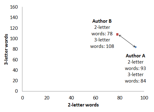
The obvious geometric distance formula, based on the Pythagorean Theorem about the length of a right-angled triangle’s sides, would give us:
With that formula, the “distance” between the two authors’ texts, as far as the distribution of two- and three-letter words goes, is about d=20.3. Nice, that’s a number, and we can say the unknown author’s text is closest to that author’s texts where this number is the smallest. There is, however, an important catch: we need to compare texts of equal length, but in reality texts come in all different sizes. If we take a sample from Author B that contains twice as many words, but the same proportion of two- and three-letter words, here’s what we get:
| Count of two-letter words | Count of three-letter words | |
| Author A | ax = 93 | ay = 84 |
| Author B | bx = 156 | by = 216 |
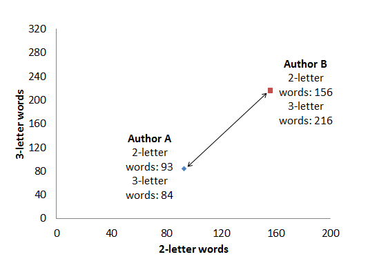
With our formula the distance is now about d=146.26, even though Author B has been meticulously producing the same proportion of two- and three-letter words, only in twice as much text. Clearly this is not what we need. We could refine our method by looking at the relative frequency of words instead: i.e., dividing every word count with the total number of words in the text. This gives us, practically, the percentage of two-letter words and three-letter words in the text at hand.
| Count of two-letter words | Count of three-letter words | |
| Author A | ax = 9.3% (93 out of 1000) | ay = 8.4% (84 out of 1000) |
| Author B | bx = 7.8% (156 out of 2000) | by = 10.8% (216 out of 2000) |
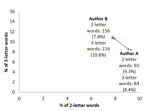
Our distance is now down to the nice approximate value of d=20.3 again, even though we are comparing a smallish and a largish orange. Consequently, converting raw counts to relative frequencies is often the first thing to do in text analysis. But it turns out a different measure comes in even more handy when comparing vectors. Let’s look at the two plots below, showing word frequencies of Author A from her 1000-word text against Author B’s word frequencies, from a smaller and a larger text:
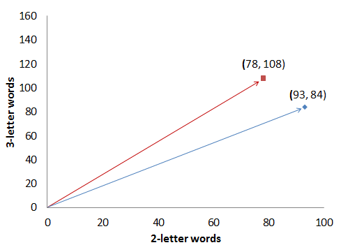
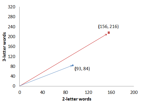
Even though both graphs show the “raw” counts, you can see that one thing stays constant: the angle of the two arrows. That angle is precisely what we’re after.
Cosine similarity and higher dimensions
For two-dimensional vectors, the cosine similarity formula gives us the cosine of the two vectors’ angle:
In plain words, that means:
- If the two arrows point in the same direction, then s equals 1. That’s as similar as you can get.
- If the two arrows point in the opposite direction, then s equals -1. That’s as different as you can get.
- If the two arrows are at right angles, then s equals 0.
- The length of the arrows doesn’t matter.
In all of the examples above, the cosine similarity of the two authors’ word frequency vectors (in our limited two-dimensional space) is approximately s=0.97788.
There is only one hyperspace jump left to do, and then the arithmetic will end. The rest of authorial analysis is a mixture of common sense and black magic. We don’t want to randomly select only two values (the frequency of two- and three-letter words) but work instead with our full 32-dimensional data in all its richness. But how do you imagine the angle between two 32-dimensional vectors?
The trick is: you don’t. You just mechanically extend the formula, feed in the numbers you’ve observed, and walk away with the results.
The cosine similarity formula above has the two dimensions hard-wired: it refers to ax and ay, and to bx and by. If instead you write a1, a2, b1 and b2 and throw in a ∑ to represent adding up stuff, it can be rewritten as:
That’s for 2 dimensions. If you need, say, n dimensions, then just do a bit of more adding up:
That’s cosine similarity for a pair of n-dimensional vectors. Welcome to Alpha Centauri.
OK, that was word length. What else?
That’s as complicated as the math gets in the whole experiment, and if you take a closer look, you can see it doesn’t go beyond adding and multiplying numbers and calculating square roots – we’re just doing a whole lot of that.
What really matters is the actual numbers we are crunching. So far I’ve kept referring to one type of data: the count (or frequency) of words that are 1, 2, 3 etc. letters long, up to 32. In his Language Log post, Patrick Juola described three additional linguistic variables that he worked with:
- The 100 most common words: what percentage of the document were “the,” what were “of,” and so on.
- The distribution of character 4-grams, groups of four adjacent characters.
- Finally, word bigrams, pairs of adjacent words.
Why do these variables seem to help identify authorship and not others? In short, that’s what I call the “black magic” of statistical methods.
How do these same variables fare for the authorial analysis of Hungarian texts? Are there other variables that may be worth looking at? And how do you know what works and what does not? To find the answers, you need to put black magic to the test of common sense. That’s what I’ll do in the next post .